Suggested posts prior to reading this one:
- A Cautionary Tale: The Bias-Variance Tradeoff in Machine Learning
- Guide: Cross Validation with Julius
Introduction
XGBoost (Extreme Gradient Boosting) is a highly efficient and effective implementation of the gradient boosting algorithm, which has gained significant popularity in the fields of machine learning and data science. It is known for its excellent performance, scalability, and ability to handle various types of data and problems, including regression, classification, and ranking tasks.
At its core, XGBoost is an ensemble learning method that combines multiple weak learners (decision trees) to create a strong and accurate predictive model. The algorithm iteratively trains decision trees on the residuals (errors) of the previous trees, gradually improving the model’s performance by minimizing a loss function.
One of the key features of XGBoost is its ability to handle missing values and automatically learn the best split points for each feature. It also employs regularization techniques to control the complexity of the trees and prevent overfitting, leading to better generalization performance on unseen data.
XGBoost has several hyperparameters that can be tuned to optimize the model’s performance, such as the number of trees, the maximum depth of each tree, the learning rate, and the regularization parameters. By carefully adjusting these hyperparameters, users can find the right balance between model complexity and generalization ability.
Example: Predicting Customer Product Purchase
To better understand how XGBoost works, let’s walk through a simple (made up) example that demonstrates the process of building decision trees and making predictions using the algorithm. Let’s consider a scenario where we want to predict whether a customer will buy a product based on their age, income, and credit score.
| Age | Income | CreditScore | BuysProduct |
|---|---|---|---|
| 25 | 50000 | 700 | 1 |
| 30 | 40000 | 650 | 0 |
| 35 | 75000 | 800 | 1 |
| 40 | 30000 | 700 | 0 |
| 45 | 60000 | 750 | 1 |
| 55 | 45000 | 600 | 0 |
Step 1: Initial assumption and residuals (learning rate = 0.1). Initial prediction = 0.5 for all instances.
What is a learning rate and why this initial assumption?
Learning Rate
The learning rate, often denoted as η, is a hyperparameter in XGBoost that controls the contribution of each tree to the final prediction. It is a value between 0 and 1 that scales the predictions of each tree before adding them to the ensemble.
The main purpose of the learning rate is to slow down the learning process and prevent the model from overfitting. By scaling down the predictions of each tree, the model takes smaller steps towards the optimal solution, allowing it to converge more smoothly and avoid overshooting the target.
A smaller learning rate (e.g., 0.1 or 0.01) generally leads to better generalization performance but requires more trees (iterations) to reach the optimal solution. On the other hand, a larger learning rate (e.g., 0.5 or 1) can lead to faster convergence but may result in a suboptimal final model.
The learning rate is a crucial hyperparameter that needs to be tuned carefully to balance the trade-off between model complexity and generalization ability.
Initial Prediction
In XGBoost, the model starts with an initial prediction, which serves as a starting point for the iterative process of building trees and updating the predictions. The initial prediction is a constant value that is assigned to all instances in the dataset.
There are several ways to determine the initial prediction:
- Global mean: A common approach is to set the initial prediction to the mean of the target variable across all instances in the training set. For example, if the target variable is binary (0 or 1), the initial prediction could be set to the proportion of positive instances in the training set.
- Prior probability: In classification problems, the initial prediction can be set to the prior probability of each class. For example, if the dataset has 60% positive instances and 40% negative instances, the initial prediction could be set to 0.6 for all instances.
- Domain knowledge: In some cases, domain knowledge or business understanding can be used to set a meaningful initial prediction. For example, if the problem is to predict the likelihood of a customer churning, and historical data suggests that the average churn rate is around 20%, the initial prediction could be set to 0.2.
- Zero: In certain scenarios, such as when the target variable is centered around zero or when the model is expected to learn the mean of the target variable through the iterative process, the initial prediction can be set to zero.
The choice of the initial prediction depends on the problem at hand and the characteristics of the dataset. In the example provided, the initial prediction is set to 0.5 for simplicity, but in practice, it would be determined based on the specific problem and dataset.
By starting with an initial prediction and iteratively adding the scaled predictions of each tree, XGBoost gradually refines the model and improves its performance. The learning rate plays a crucial role in controlling the contribution of each tree and ensuring a smooth and controlled learning process.
| Age | Income | CreditScore | BuysProduct | InitialPrediction | PseudoResidual |
|---|---|---|---|---|---|
| 25 | 50000 | 700 | 1 | 0.5 | 0.5 |
| 30 | 40000 | 650 | 0 | 0.5 | -0.5 |
| 35 | 75000 | 800 | 1 | 0.5 | 0.5 |
| 40 | 30000 | 700 | 0 | 0.5 | -0.5 |
| 45 | 60000 | 750 | 1 | 0.5 | 0.5 |
| 55 | 45000 | 600 | 0 | 0.5 | -0.5 |
What is a pseudo residual?
In XGBoost, the term “pseudo-residuals” is used instead of just “residuals” because the residuals are not calculated in the same way as in traditional regression models.
In a typical regression setting, residuals are defined as the difference between the observed values and the predicted values.
However, in XGBoost and other gradient boosting algorithms, the residuals are calculated based on the negative gradient of the loss function with respect to the predicted values. This is why they are called “pseudo-residuals” or “gradient residuals.”
Step 2: First tree to predict initial residuals (lambda = 0) (just a simplified example of what it might start like). Tree depth is another model parameter that the user needs to optimize later on).
What is lambda (λ)?
In XGBoost classification, the lambda term, also known as the regularization parameter, helps control the model’s complexity and plays a crucial role in managing the bias-variance tradeoff.
A higher lambda value introduces more regularization, which constrains the model’s weights and reduces its complexity. This increased regularization helps to mitigate overfitting by adding a penalty term to the objective function, discouraging the model from fitting noise in the training data. As a result, a model with strong regularization tends to have higher bias but lower variance.
Conversely, a lower lambda value allows the model to have more flexibility in fitting the training data. This can lead to a more complex model that captures intricate patterns in the data, resulting in lower bias. However, this increased complexity also makes the model more prone to overfitting, leading to higher variance.
By tuning the lambda parameter, you can find the right balance between bias and variance for your specific problem. The optimal lambda value depends on factors such as the size and complexity of your dataset, the noise level, and the desired generalization performance.
In summary, the lambda term in XGBoost classification serves as a regularization mechanism that helps control the model’s complexity and manage the bias-variance tradeoff, enabling you to find the sweet spot between underfitting and overfitting for your particular task.
Note: In a decision tree, all final values that have nothing branching out of them are called leaves.
          CreditScore <= 700
          /                \
     Income <= 45000    [0.5, 0.5]
      /             \
[-0.5, -0.5, -0.5] [0.5]
Similarity Score:
For a binary classification using logistic regression, where the output is modeled as the probability of the positive class, the leaf output (or the probability that specific leaf adds to the overall prediction) is calculated like this:

Using that formula, I can see for example that if the CreditScore is less than or equal to 700 and income is less than or equal to 45000, we have three residuals, -0.5, -0.5 and -0.5. Plugging them into the leaf output equation gives us 1.29. Similarly for the remaining leaves we get 0.20 and 0.67.
These outputs will be used to update the previous predictions.
We will now calculate the leaf outputs using the residuals for each group and update the predictions. Based on this updated prediction, we will recalculate the residuals. The learning rate (η) typically used by XGBoost for updates can be set to 0.1 for demonstration purposes, but it’s adjustable based on the specific scenario. Let’s calculate these updated predictions and new residuals.

For Left Leaf (CreditScore ≤ 700 & Income ≤ 45000)
- New Predictions:
[0.479, 0.479, 0.479](approximately) - New Residuals:
[-0.479, -0.479, -0.479](approximately)
For Right Leaf (CreditScore ≤ 700 & Income > 45000)
- New Prediction:
[0.510](approximately) - New Residual:
[0.490](approximately)
For Right Child (CreditScore > 700)
- New Predictions:
[0.517, 0.517](approximately) - New Residuals:
[0.483, -0.517](assuming actual values of 1 for the first and 0 for the second)
Here’s how the updated table would look with the old and new predictions and residuals:
| Age | Income | CreditScore | BuysProduct | InitialPrediction | OldPseudoResiduals | NewPrediction | NewPseudoResiduals |
|---|---|---|---|---|---|---|---|
| 25 | 50000 | 700 | 1 | 0.5 | 0.5 | 0.510 | 0.490 |
| 30 | 40000 | 650 | 0 | 0.5 | -0.5 | 0.479 | -0.479 |
| 35 | 75000 | 800 | 1 | 0.5 | 0.5 | 0.517 | 0.483 |
| 40 | 30000 | 700 | 0 | 0.5 | -0.5 | 0.479 | -0.479 |
| 45 | 60000 | 750 | 1 | 0.5 | 0.5 | 0.517 | 0.483 |
| 55 | 45000 | 600 | 0 | 0.5 | -0.5 | 0.479 | -0.479 |
Notice how the residuals went down compared to the previous ones, and the predictions came closer to the truth? That’s because in the gradient boosting framework, each tree incrementally improves the predictions by learning from the residuals of the previous trees. Essentially, each tree is trained to predict the gradient of the loss function with respect to the predictions, hence refining the model by correcting errors iteratively. This systematic reduction of residuals is aimed at minimizing the overall prediction error in a step-by-step manner.
How does the model select the root of each tree?
The model selects the root of each tree based on the Gain, which is a metric used to quantify the improvement in prediction accuracy achieved by a potential split. Specifically, Gain is calculated as the difference in similarity scores between a node before splitting and the sum of similarity scores of the nodes after the split. The split that provides the highest Gain is selected as the root of the new tree, as it maximally reduces uncertainty and error in the predictions within those groups.

Gain, therefore, guides the construction of the tree by choosing splits that offer the most significant increase in prediction precision. This approach ensures that the trees in the boosting process are built in a way that continuously focuses on the hardest-to-predict instances, which is evident from the gradient nature of the algorithm where each tree is built to improve upon the shortcomings of its predecessors.
The similarity score measures the homogeneity of a node. A higher score indicates a more accurate prediction for the data points within that node. Previous probability is the predicted probability from the previous iteration (0.5 for all in the initial iteration). λ is a regularization parameter that helps prevent overfitting (assume λ=1 for simplicity). This structured approach to building each tree ensures that the ensemble model converges efficiently to a strong predictive performance, capitalizing on systematic, gradient-driven corrections.

After Step 2, the model keeps creating trees and incrementally improving the predictions until a desired endpoint is reached. This endpoint can be determined by several criteria, such as:
- Number of Trees (n_estimators): A predefined number of trees are built, with each tree attempting to correct the residuals left by its predecessors. Once this number is reached, the building of new trees stops.
- Performance Threshold: The training process can be halted if the model reaches a performance metric that satisfies the requirements, such as a specific accuracy or error rate on a validation dataset.
- Minimal Gain: If subsequent trees contribute an insignificant improvement in performance (i.e., the gain from new splits is below a predetermined threshold), the training may stop to prevent overfitting and to conserve computational resources.
- Early Stopping: A more dynamic criterion where the model training stops if the validation score does not improve for a given number of consecutive trees. This technique helps in preventing overfitting and ensures that the model is optimal in terms of generalization to new data.
By using one or a combination of these stopping criteria, the model ensures that it neither underfits nor overfits, maintaining a balance between bias and variance, thus optimizing the predictive performance on unseen data.
Using Julius
Now that we understand some of the basics behind XGBoost (for classification), let’s explore how quickly and easily Julius can help us prepare the data and train a model to do what I have just painstakingly done by hand. The task remains the same - build classification trees that are very good at predicting a given dependent variable when all of their predictions combine.
The dataset used contains bank customers using a specific credit card service. Some of them have left it this service and our goal is to predict who is likely to leave so that we can inform our imaginary manager and potentially build some sort of campaign aimed at getting them to stay.
What’s really important with XGBoost is that we can only give it integers, floats or true/false columns. Basically, numbers only. What I love about Julius is how quickly I can get it to perform a very tedious amount of Python work. It immediately understand the dataset really well:

As you can see, there is a column called CLINETNUM which is the unique ID for each client and worthless to our model as it contains no predictive power. I asked Julius to drop it and to describe the dependent variable (the one we are trying to predict) to me. That is the Attrition_Flag variable. From the Julius summary, I can immediately tell that only ~16% of customers have closed their accounts meaning that we have an imbalanced dataset - a dataset where the ratio of 1s to 0s in the dependent variable is not close to 1. Additionally, we seem to have a lot of non-numeric columns.
To clean these columns, I would first like a visual inspection of all the categorical ones, so that I can tell Julius how to clean them.
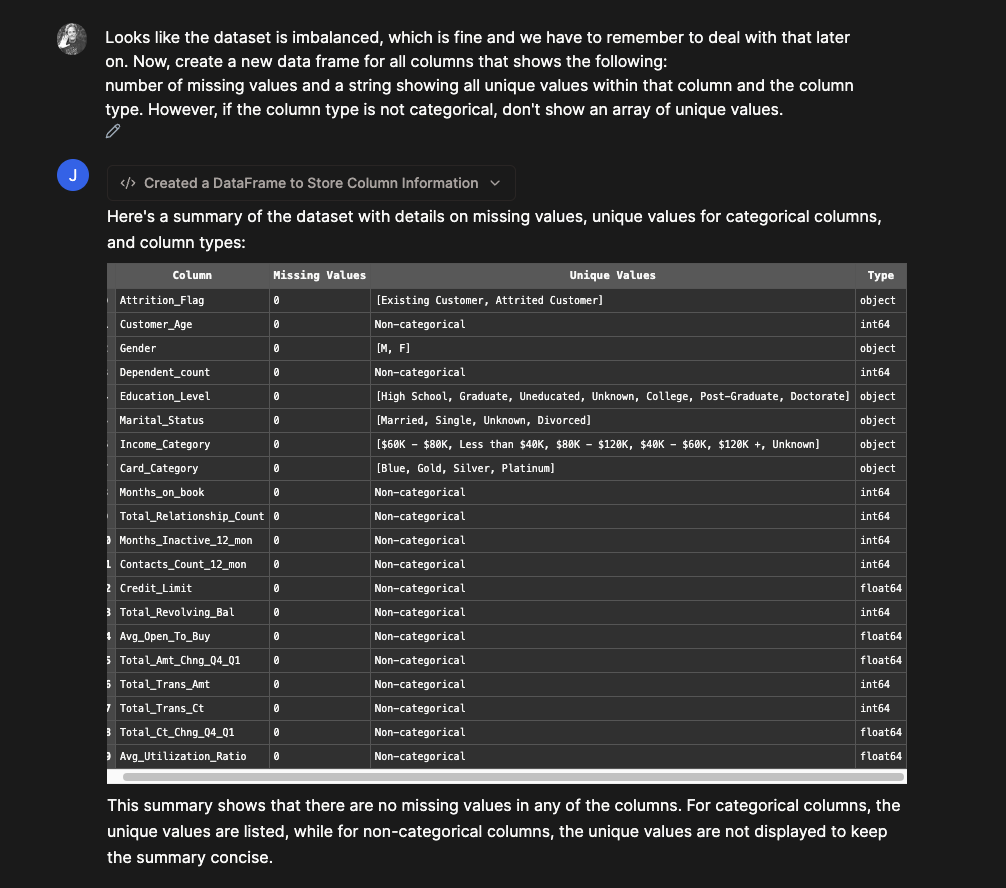
Code that Julius wrote
# Create a new dataframe to display the number of missing values, unique values (for categorical columns), and column types
summary_df = pd.DataFrame(columns=['Column', 'Missing Values', 'Unique Values', 'Type'])

for col in df.columns:
    col_data = df[col]
    col_type = col_data.dtype
    missing_values = col_data.isnull().sum()
    unique_values = col_data.unique() if col_data.dtype == 'object' else 'Non-categorical'
    summary_df = summary_df.append({'Column': col, 'Missing Values': missing_values, 'Unique Values': unique_values, 'Type': col_type}, ignore_index=True)

print(summary_df)
This is the perfect way to quickly inspect and give instructions. In two more quick prompts, I have a finalized dataset. Julius helped me one-hot encode the categorical variables and clean up some column names and text so that the XGBoost classifier does not break accidentally later on.

What is one-hot encoding?
One hot encoding is a technique used to convert categorical variables into a numerical representation that machine learning algorithms can easily understand and process. It creates a binary vector for each unique category in a categorical feature, where each element of the vector represents a specific category and takes the value of 1 if the instance belongs to that category, and 0 otherwise.
Here’s a quick example to illustrate one hot encoding:
Suppose we have a dataset with a categorical feature “Color” that can take three different values: Red, Green, and Blue.
Original data:
| Instance | Color |
|---|---|
| 1 | Red |
| 2 | Green |
| 3 | Blue |
| 4 | Red |
| 5 | Green |
After applying one hot encoding, the “Color” feature will be transformed into three separate binary features, one for each unique category:
One hot encoded data:
| Instance | Color_Red | Color_Green | Color_Blue |
|---|---|---|---|
| 1 | 1 | 0 | 0 |
| 2 | 0 | 1 | 0 |
| 3 | 0 | 0 | 1 |
| 4 | 1 | 0 | 0 |
| 5 | 0 | 1 | 0 |
In the one hot encoded representation, each instance has a value of 1 in the corresponding category’s column and 0 in the other columns. This encoding allows machine learning algorithms to treat categorical variables as numerical features, enabling them to process and learn from the data effectively.
One hot encoding is widely used in various machine learning tasks, such as linear regression, logistic regression, and neural networks, where categorical variables need to be transformed into a suitable numerical representation.
Now is the time to split the data and train a Classifier. First, due to the imbalance I mentioned earlier, I want to make sure that, for the training and the testing datasets, Julius uses stratified sampling which will ensure that when sampling it maintains the same proportion of each class as in the original dataset. This is crucial because if the model is trained on a dataset with a significantly different class distribution than the test set, it may lead to biased and unreliable performance metrics.

Code that Julius wrote
# Splitting the data into independent and dependent variables
X = encoded_df.drop('Attrition_Flag', axis=1)
y = encoded_df['Attrition_Flag']

# Importing train_test_split from sklearn
from sklearn.model_selection import train_test_split

# Performing a stratified train-test split
X_train, X_test, y_train, y_test = train_test_split(X, y, test_size=0.2, random_state=42, stratify=y)

# Calculating the percentage of attrition in train and test datasets
attrition_percent_train = y_train.value_counts(normalize=True) * 100
attrition_percent_test = y_test.value_counts(normalize=True) * 100

print('Attrition percentage in training set:', attrition_percent_train)
print('Attrition percentage in test set:', attrition_percent_test)
We have arrived at the best part - training the model. I am going to ask for a specific random seed (so that my work can be replicated by others), I am going to tell the model to use a binary:logistic objective (much like in the simplified example above, we are trying to classify 1s and 0s) and I am going to tell it to stop if there are no significant training improvements after 10 consecutive trees.

Code that Julius wrote
# Install xgboost if not already installed
!pip install xgboost==1.6.2

# Importing XGBClassifier from xgboost
from xgboost import XGBClassifier

# Creating the XGBClassifier model with specified parameters
model = XGBClassifier(objective='binary:logistic', seed=123, eval_metric='aucpr', verbosity=1)

# Fitting the model with early stopping
model.fit(X_train, y_train, eval_set=[(X_test, y_test)], early_stopping_rounds=10, verbose=True)
Note: Telling Julius to install a specific library is just my preference to avoid Julius having to figure out that it needs to install it. But no worries, if you forget that step, Julius will figure it out without issues.
We can see in the output what I have attempted to explain in the simple example above. The model trains by creating trees that each improve upon the previous by focusing on predicting its residuals using a predefined loss function. In this case I chose AUCPR based on XGBoost documentation that suggests this approach for imbalanced datasets.
What is AUCPR?
AUCPR stands for Area Under the Precision-Recall Curve. It is an evaluation metric used to assess the performance of a binary classification model, particularly in imbalanced datasets where the positive class is rare compared to the negative class.
The Precision-Recall curve is a plot that shows the relationship between precision and recall at different classification thresholds. Precision measures the proportion of true positive predictions among all positive predictions, while recall (also known as sensitivity or true positive rate) measures the proportion of true positive predictions among all actual positive instances.
The AUCPR is calculated by computing the area under the Precision-Recall curve. It provides a single scalar value that summarizes the model’s performance across all possible classification thresholds. A higher AUCPR indicates better performance, with a perfect classifier achieving an AUCPR of 1.
The AUCPR is particularly useful in scenarios where the focus is on correctly identifying the positive instances (e.g., detecting fraudulent transactions, identifying rare diseases), and the cost of false positives is relatively high. In such cases, a model with high precision is desirable, even if it sacrifices some recall.
Here are a few key points about AUCPR:
- It is sensitive to class imbalance: AUCPR is especially relevant when dealing with imbalanced datasets because it focuses on the performance of the minority (positive) class.
- It prioritizes precision: AUCPR emphasizes the importance of precision, which is crucial when the cost of false positives is high.
- It is threshold-independent: AUCPR summarizes the model’s performance across all possible classification thresholds, providing a comprehensive evaluation.
- It is different from AUROC: AUCPR should not be confused with AUROC (Area Under the Receiver Operating Characteristic curve), which is another common metric for binary classification. AUROC considers both true positive rate and false positive rate, while AUCPR focuses on precision and recall.
When evaluating classifiers on imbalanced datasets, it is recommended to use AUCPR in conjunction with other metrics like precision, recall, and F1 score to get a comprehensive understanding of the model’s performance.
I have mostly let Julius run with the default parameters for XGBoost classifier. However, there are many of those! One approach (that I won’t do here to limit the scope of this post) would be to tell Julius to explore 3 different values for some key parameters like the regularization lambda and the learning rate mentioned above, or the tree depth or gamma (used for pruning the trees) and to perform a GridSearch cross validation and find the most optimal parameter combination for this dataset. That would take some time and I will avoid for now.
However, we have one simple approach to improving this model. Let’s think back to what it is meant to do: we want to know which customers are about to stop using the credit card service (or churn) so we really want to make sure this model is good at detecting those. We are not so concerned about incorrectly predicting people who are going to stay and then bothering them with out campaign designed to prevent churn. So first, let’s get a Confusion Matrix from Julius and see how well this initial model performed.

There are a lot of people who remained customers and we correctly predicted they would (1679). We also did quite a good job at predicting those that would cancel their service that indeed canceled their service (276). What is bothering me somewhat is the 49 people we missed and classified incorrectly. I would like to lower that number.
By setting the scale_pos_weight, you effectively tell the model how much more importance it should give to the minority class. A common practice is to set this parameter to the ratio of the number of negative instances to the number of positive instances. This helps in pushing the model to pay more attention to the positive class. In our case, that ratio is about 5. The parameter works by scaling the gradient terms for the positive class during the calculation of the loss during training. By increasing the weight of the positive class, the loss due to errors in predicting the positive class instances becomes more significant, thus encouraging the model to correct these errors preferentially.
So let’s implement it and print the new confusion matrix.

Success! We have improved our prediction on the relevant group. I will stop here but please feel free to experiment with this model and data.
What does an actual tree look like?
In the initial example, I manually constructed a very simple tree, from a very small dataset. However, in practice, the trees can get quite complex. Here is the very first tree constructed by the model Julius built:

this is the first root selected by the algorithm as the one maximizing leaf purity
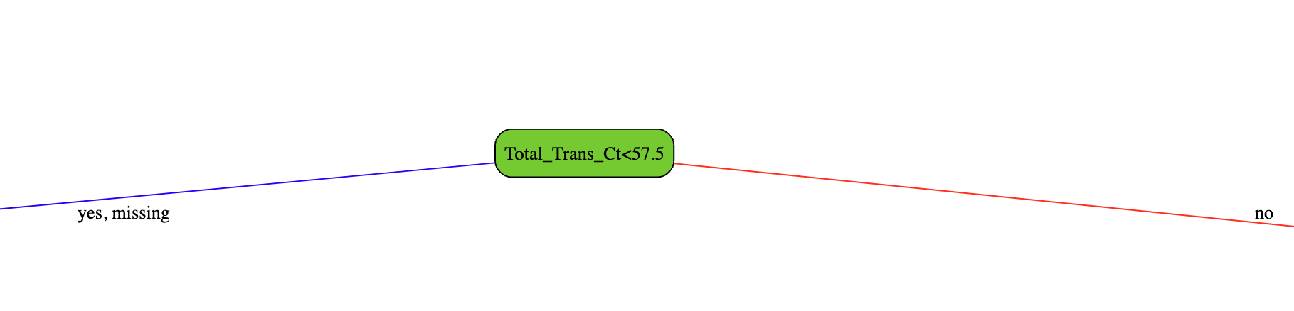
and here are some leaf output values (that then get further reduced by the learning rate to allow the model to take small steps)

Conclusion
In this post, we have explored the powerful XGBoost algorithm and its ability to build accurate and efficient predictive models. We started with a simple example to understand the core concepts behind XGBoost, such as decision trees, pseudo-residuals, learning rate, and how the algorithm selects the best splits based on gain and similarity scores.
We then dove into a real-world problem of predicting customer churn for a credit card service using a dataset from Kaggle. Thanks to the assistance of Julius we were able to quickly and easily prepare the data, handle categorical variables through one-hot encoding, and ensure a balanced representation of classes in the training and testing sets using stratified sampling.
By training an XGBoost classifier with Julius, we demonstrated how to specify important parameters, evaluate the model’s performance using the AUCPR metric, and interpret the results through a confusion matrix. We also learned how to tackle class imbalance by adjusting the scale_pos_weight parameter, which significantly improved our model’s ability to correctly identify customers likely to churn.
Finally, we visualized an actual decision tree constructed by the trained XGBoost model, providing insights into how the algorithm selects the most informative features and splits the data to make predictions.
This post has shown that XGBoost, coupled with the power of AI assistants like Julius, can be a valuable tool in a data scientist’s arsenal. By understanding the underlying principles and leveraging the right tools, we can build robust and accurate models to solve complex real-world problems. As we continue to explore the vast landscape of machine learning, XGBoost will undoubtedly remain a go-to algorithm for its performance, flexibility, and interpretability.
Thank you @rahul and Julius team for building this amazing tool!
Keywords: AI, XGBoost, Julius, Gradient Boosting, Decision Trees, Machine Learning, Data Science, Binary Classification, Imbalanced Datasets, Stratified Sampling, One-Hot Encoding, Confusion Matrix, AUCPR, Pseudo-Residuals, Regularization, Kaggle, Customer Churn Prediction, Python, Scikit-learn.
